YOLOv4 from scratch

YOLOv3

Bounding Box

YOLOv2 부터 Anchor box(prior box)를 미리 설정하여 최종 bounding box 예측에 활용한다. 위 그림에서는 $b_x, b_y, b_w, b_h$가 최종적으로 예측하고자 하는 bounding box이다. 검은 점선은 사전에 설정된 Anchor box로 이 Anchor box를 조정하여 파란색의 bounding box를 예측하도록 한다.

모델은 직접적으로 $b_x, b_y, b_w, b_h$ 를 예측하지 않고 $t_x, t_y, t_w, t_h$를 예측하게 된다. 범위제한이 없는 $t_x, t_y$ 에 sigmoid($\sigma$)를 적용해주어 0과 1사의 값으로 만들어주고, 이를 통해 bbox의 중심 좌표가 1의 크기를 갖는 현재 cell을 벗어나지 않도록 해준다. 여기에 offset인 $c_x, c_y$를 더해주면 최종적인 bbox의 중심 좌표를 얻게 된다.

$b_w, b_h$의 경우 미리 정해둔 Anchor box의 너비와 높이를 얼만큼의 비율로 조절할 지를 Anchor와 $t_w, t_h$에 대한 log scale을 이용해 구한다.

YOLOv2에서는 bbox를 예측할 때 $t_x, t_y, t_w, t_h$를 예측한 후 그림에서의 $b_x, b_y, b_w, b_h$로 변형한 뒤 $L_2$ loss를 통해 학습시켰지만, YOLOv3에서는 ground truth의 좌표를 거꾸로 $\hat{t}_ {∗}$로 변형시켜 예측한 $t_{∗}$와 직접 $L_1$ loss로 학습시킨다. ground truth의 $x, y$좌표의 경우 아래와 같이 변형되고,

\[\begin{aligned}&b_{∗}= \sigma(\hat{t}_ {∗}) + c_{∗}\\ &\sigma(\hat{t}_ {∗}) = b_{∗} - c_{∗}\\ &\hat{t}_ {∗} = \sigma^{-1}(b_{∗} - c_{∗})\end{aligned}\]

$w, h$는 아래와 같이 변형된다.

\[\hat{t}_ {∗} = \ln\left(\frac{b_{∗}}{p_{∗}}\right)\]

결과적으로 $x, y, w, h$ loss는 ground truth인 $\hat{t}_ {∗}$ prediction value인 ${t}_ {∗}$사이의 차이 $\hat{t}_ {∗} - {t}_ {∗}$를 통한 Sum-Squared Error(SSE)로 구해진다.

Model

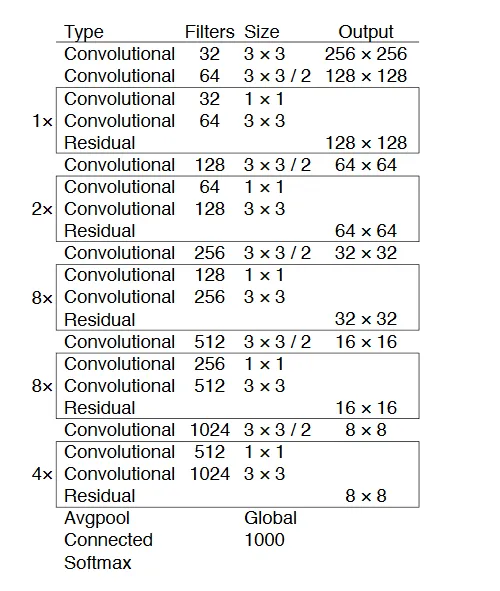
모델의 backbone은 $3 \times 3$, $1 \times 1$ Residual connection을 사용하면서 최종적으로 53개의 conv layer를 사용하는 Darknet-53 을 이용한다. Darknet-53의 Residual block안에서도 bottleneck 구조를 사용하며, input의 channel을 중간에 반으로 줄였다가 다시 복구시키는데 이렇게 하므로써 연산량을 줄일 수 있다. 이때 Residual block의 $1 \times 1$ conv는 $s=1, p=0$ 이고, $3 \times 3$ conv는 $s=1, p=1$이다.

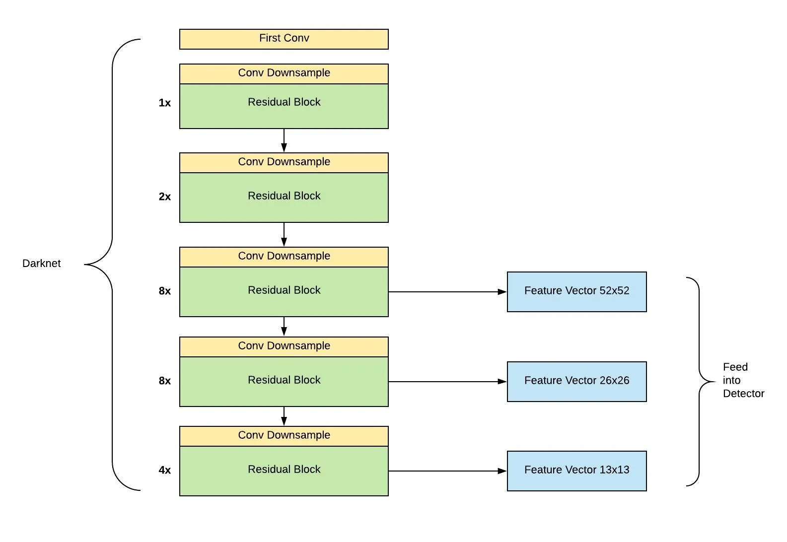
YOLOv3 model의 특징은 물체의 scale을 고려하여 3가지 크기의 output이 나오도록 FPN과 유사하게 설계하였다는 것이다. 오른쪽 그림과 같이 $416 \times 416$의 크기를 feature extractor로 받았다고 하면, feature map이 크기가 $52 \times 52$, $26 \times 26$, $13 \times 13$이 되는 layer에서 각각 feature map을 추출한다.

그 다음 가장 높은 level, 즉 해상도가 가장 낮은 feature map부터 $1 \times 1$, $3 \times 3$ conv layer로 구성된 작은 Fully Convolutional Network(FCN)에 입력한다. 이후 이 FCN의 output channel이 512가 되는 시점에서 feature map을 추출한 뒤, $2\times$로 upsampling을 진행한다. 이후 바로 아래 level에 있는 feature map과 concatenate를 해주고, 이렇게 만들어진 merged feature map을 다시 FCN에 입력한다. 이 과정을 다음 level에도 똑같이 적용해주고 이렇게 3개의 scale을 가진 feature map이 만들어진다. 각 scale에 따라 나오는 최종 feature map의 형태는 $N \times N \times \left[3 \cdot (4+1+80)\right]$이다. 여기서 $3$은 grid cell당 predict하는 anchor box의 수를, $4$는 bounding box offset $(x, y, w, h)$, $1$은 objectness prediction, $80$은 class의 수 이다. 따라서 최종적으로 얻는 feature map은 $\left[52 \times 52 \times 255\right], \left[26 \times 26 \times 255\right], \left[13 \times 13 \times 255\right]$이다.

이러한 방법을 통해 더 높은 level의 feature map으로부터 fine-grained 정보를 얻을 수 있으며, 더 낮은 level의 feature map으로부터 더 유용한 semantic 정보를 얻을 수 있다.

Loss Function

\[λ_ {coord} \sum_ {i=0}^{S^2} \sum_ {j=0}^B 𝟙^{obj}_ {i j} \left[(t_ {x_ i} - \hat{t_ {x_ i}})^2 + (t_ {y_ i} - \hat{t_ {y_ i}})^2 \right] \\ +λ_ {coord} \sum_ {i=0}^{S^2} \sum_ {j=0}^B 𝟙^{obj}_ {i j} \left[(t_ {w_ i} - \hat{t_ {w_ i}})^2 + (t_ {h_ i} - \hat{t_ {h_ i}})^2 \right] \\ +\sum_{i=0}^{S^2} \sum_{j=0}^B 𝟙^{obj}_{i j} \left[-(o_i\log(\hat{o_i}) + (1 - o_i)\log(1 - \hat{o_i}))\right] \\ +Mask_{ig} \cdot λ_{noobj} \sum_{i=0}^{S^2} \sum_{j=0}^B 𝟙^{noobj}_{i j} \left[-(o_i\log(\hat{o_i}) + (1 - o_i)\log(1 - \hat{o_i}))\right] \\ +\sum_{i=0}^{S^2} \sum_{j=0}^B 𝟙^{obj}_ {i j} \sum_{c \in classes} \left[-(c_i\log(\hat{c_i}) + (1 - c_i)\log(1 - \hat{c_i}))\right]\]

$S$ : number of cells

$B$ : number of anchors

$o$ : objectness

$c$ : class label

$λ_ {coord}$ : coordinate loss balance constant

$λ_{noobj}$ : no confidence loss balance constant

$𝟙^{obj}_ {i j}$ : 1 when there is object, 0 when there is no object

$𝟙^{noobj}_ {i j}$ : 1 when there is no object, 0 when there is object

$Mask_{ig}$ : tensor that masks only the anchor with iou $\le$ 0.5. Have a shape of $\left[S, S, B\right]$.

각각의 box는 multi-label classification을 하게 되는데 논문에서는 softmax가 성능이 좋지 못하기 때문에, binary cross-entropy loss를 사용했다고 한다. 하나의 box안에 복수의 객체가 존재하는 경우 softmax는 적절하게 객체를 알아내지 못하기 때문에, box 안에 각 class가 존재하는 여부를 확인하는 binary cross-entropy가 보다 적절하다고 할 수 있다.

$o$ (objectness)는 anchor와 bbox의 iou가 가장 큰 anchor의 값이 1, 그렇지 않은 경우의 값이 0인 $\left[N, N, 3, 1\right]$의 tensor로 만들어진다. $c$ (class label)은 one-encoding으로 $\left[N, N, 3, n \right]$ ($n$ : num_classes) 의 shape를 갖는 tensor로 만들어진다.

YOLOv4

Model

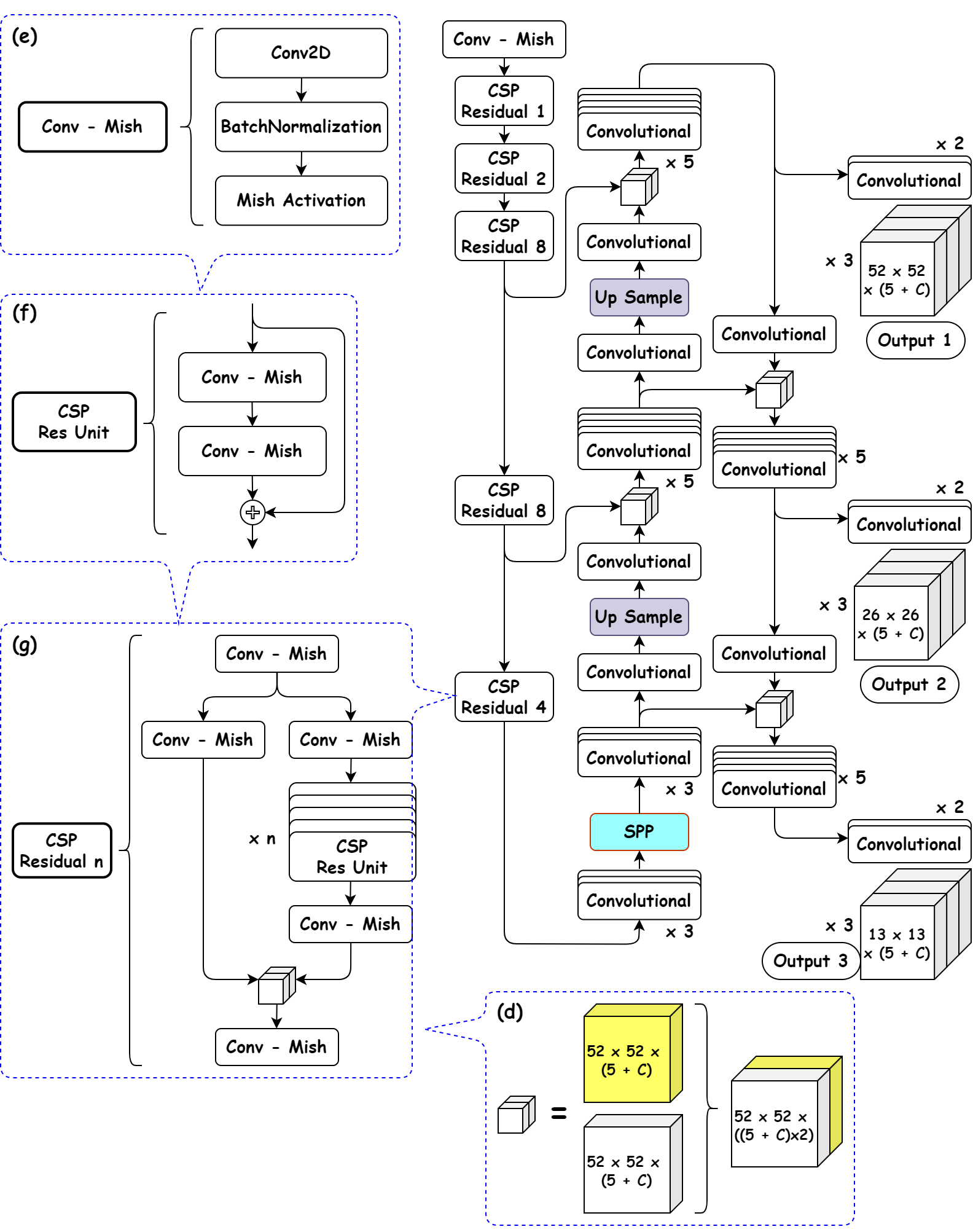
전체적인 구조는 YOLOv3과 유사하지만 YOLOv4는 CSPDarknet53+SPP를 사용한다. CSPDarknet53은 Darknet53에 CSPNet을 적용한 것이다. CSPNet은 위 사진의 CSP Residual 부분과 같이 base layer의 feature map을 두 개로 나눈 뒤($X_0 \to X_0^{‘}, X_0^{‘’}$) $X_0^{‘’}$는 Dense Layer에 통과 시키고 $X_0^{‘}$는 그대로 가져와서 마지막에 Dense Layer의 출력값인 ($X_0^{‘’}, x_1, x_2, …$)을 transition layer에 통과시킨 $X_T$와 concat시킨다. 이후 concat된 결과가 다음 transition layer를 통과하면서 $X_U$가 생성된다.

\[\begin{aligned}X_k &= W_K^{ * }[X_0^{''}, X_1, ..., X_{k-1}]\\ X_T &= W_T^{ * }[X_0^{''}, X_1, ..., X_{k}]\\ X_U &= W_U^{ * }[X_0^{'}, X_T]\\ \end{aligned}\] \[\begin{aligned}W_k^{'} &= f(W_k, g_0^{''}, g_1, g_2, ..., g_{k-1})\\  W_T^{'} &= f(W_T, g_0^{''}, g_1, g_2, ..., g_{k})\\  W_U^{'} &= f(W_U, g_0^{'}, g_T)\\      \end{aligned}\]

이렇게 하므로써 CSPDenseNet은 DenseNet의 feature reuse 특성을 활용하면서, gradient flow를 truncate($X_0 \to X_0^{‘}, X_0^{‘’}$)하여 과도한 양의 gradient information 복사를 방지할 수 있다.

Box Loss

일반적으로 IoU-based loss는 다음과 같이 표현된다.

\[L = 1 - IoU + \mathcal{R}(B, B^{gt})\]

여기서 $R(B, B^{gt})$는 predicted box $B$와 target box $B^{gt}$에 대한 penalty term이다.

$1 - IoU$로만 Loss를 구할 경우 box가 겹치지 않는 case에 대해서 어느 정도의 오차로 교집합이 생기지 않은 것인지 알 수 없어서 gradient vanishing 문제가 발생했다. 이러한 문제를 해결하기 위해 penalty term을 추가한 것이다.

Generalized-IoU(GIoU)

Generalized-IoU(GIoU) 의 경우 Loss는 다음과 같이 계산된다.

\[L_{GIoU} = 1 - IoU + \frac{|C - B ∪ B^{gt}|}{|C|}\]

여기서 $C$는 $B$와 $B^{gt}$를 모두 포함하는 최소 크기의 Box를 의미한다. Generalized-IoU는 겹치지 않는 박스에 대한 gradient vanishing 문제는 개선했지만 horizontal과 vertical에 대해서 에러가 크다. 이는 target box와 수평, 수직선을 이루는 Anchor box에 대해서는 $\vert C - B ∪ B^{gt} \vert$가 매우 작거나 0에 가까워서 IoU와 비슷하게 동작하기 때문이다. 또한 겹치지 않는 box에 대해서 일단 predicted box의 크기를 매우 키우고 IoU를 늘리는 동작 특성 때문에 수렴 속도가 느리다.

Distance-IoU(DIoU)

GIoU가 면적 기반의 penalty term을 부여했다면, DIoU는 거리 기반의 penalty term을 부여한다. DIoU의 penalty term은 다음과 같다.

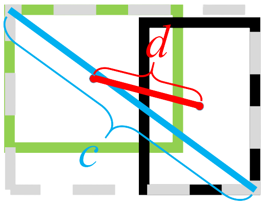
\[\mathcal{R}_{DIoU} = \frac{\rho^2(b, b^{gt})}{c^2}\]

$\rho^2$는 Euclidean거리이며 $c$는 $B$와 $B^{gt}$를 포함하는 가장 작은 Box의 대각선 거리이다.

DIoU Loss는 두 개의 box가 완벽히 일치하면 0, 매우 멀어지면 $L_{GIoU} = L_{DIoU} \to 2$가 된다. 이는 IoU가 0이 되고, penalty term이 1에 가깝게 되기 때문이다. Distance-IoU는 두 box의 중심 거리를 직접적으로 줄이기 때문에 GIoU에 비해 수렴이 빠르고, 거리기반이므로 수평, 수직방향에서 또한 수렴이 빠르다.

DIoU-NMS

DIoU를 NMS(Non-Maximum Suppression)에도 적용할 수 있다. 일반적인 NMS의 경우 이미지에서 같은 class인 두 물체가 겹쳐있는 Occlusion(가림)이 발생한 경우 올바른 박스가 삭제되는 문제가 발생하는데, DIoU를 접목할 경우 두 박스의 중심점 거리도 고려하기 때문에 target box끼리 겹쳐진 경우에도 robust하게 동작할 수 있다.

\[s_i =\begin{cases}s_ i, & IoU - \mathcal{R}_ {DIoU}(\mathcal{M}, B_i) < \epsilon\\0, & IoU - \mathcal{R}_{DIoU}(\mathcal{M}, B_i) \ge \epsilon\end{cases}\]

가장 높은 Confidence score를 갖는 $\mathcal{M}$에 대해 IoU와 DIoU의 distance penalty를 동시에 고려하여 IoU가 매우 크더라도 중심점 사이의 거리가 멀면 다른 객체를 탐지한 것일 수도 있으므로 위와 같이 일정 임계치 $\epsilon$ 보다 작으면 없애지 않고 보존한다.

Complete-IoU(CIoU)

DIoU, CIoU를 제안한 논문에서 말하는 성공적인 Bounding Box Regression을 위한 3가지 조건은 overlap area, central point distance, aspect ratio이다. 이 중 overlap area, central point는 DIoU에서 이미 고려했고 여기에 aspect ratio를 고려한 penalty term을 추가한 것이 CIoU이다. CIoU penalty term는 다음과 같이 정의된다.

\[\mathcal{R}_{CIoU} = \frac{\rho^2(b, b^{gt})}{c^2} + \alpha v \\ v = \frac{4}{π^2}(\arctan{\frac{w^{gt}}{h^{gt}}} - \arctan{\frac{w}{h}})^2 \\ \alpha = \frac{v}{(1 - IoU) + v}\]

$v$의 경우 bbox는 직사각형이고 $\arctan{\frac{w}{h}} = \theta$이므로 $\theta$의 차이를 통해 aspect ratio를 구하게 된다. 이때 $v$에 $\frac{2}{π}$가 곱해지는 이유는 $\arctan$ 함수의 최대치가 $\frac{2}{π}$ 이므로 scale을 조정해주기 위해서이다.

$\alpha$는 trade-off 파라미터로 IoU가 큰 box에 대해 더 큰 penalty를 주게 된다.

CIoU에 대해 최적화를 수행하면 아래와 같은 기울기를 얻게 된다. 이때, $w, h$는 모두 0과 1사이로 값이 작아 gradient explosion을 유발할 수 있다. 따라서 실제 구현 시에는 $\frac{1}{w^2 + h^2} = 1$로 설정한다.

\[\frac{\partial v}{\partial w} = \frac{8}{π^2}(\arctan{\frac{w^{gt}}{h^{gt}}} - \arctan{\frac{w}{h}}) \times \frac{h}{w^2 + h^2} \\ \frac{\partial v}{\partial h} = -\frac{8}{π^2}(\arctan{\frac{w^{gt}}{h^{gt}}} - \arctan{\frac{w}{h}}) \times \frac{w}{w^2 + h^2}\]

Cosine Annealing

\[\eta_t = \eta_{\min} + \frac{1}{2}(\eta_{\max} - \eta_{\min})\left(1 + \cos{\left(\frac{T_{cur}}{T_{\max}}\pi\right)} \right), \ T_{cur} \neq (2k+1)T_{\max}\]

$\eta_{\min}$ : min learning rate

$\eta_{\max}$ : max learning rate

$T_{\max}$ : period

YOLOv4 Implementation

    

전체적인 틀은 Aladdin Persson의 라이브러리를 참고하였고, YOLOv4 model은 논문과 YOLOv4 diagram에 기반하여 직접 구현해보았다.

Blocks

class DarknetConv2D(nn.Module):
    def __init__(self, in_channels, out_channels, kernel_size, stride, act="mish", bn_act=True):
        super().__init__()

        padding = (kernel_size - 1) // 2

        self.conv = nn.Conv2d(
            in_channels=in_channels, out_channels=out_channels,
            kernel_size=kernel_size, stride=stride, padding=padding,
            bias=not bn_act
        )

        self.bn = nn.BatchNorm2d(out_channels)
        self.mish = nn.Mish()
        self.leaky = nn.LeakyReLU(0.1, inplace=True)
        self.use_bn_act = bn_act
        self.act = act

    def forward(self, x):
        if self.use_bn_act:
            if self.act == "mish":
                return self.mish(self.bn(self.conv(x)))
            elif self.act == "leaky":
                return self.leaky(self.bn(self.conv(x)))
        else:
            return self.conv(x)

class CSPResBlock(nn.Module):
    def __init__(self, in_channels, is_first=False, num_repeats=1):
        super().__init__()

        self.route_1 = DarknetConv2D(in_channels, in_channels//2, 1, 1, 'mish')
        self.route_2 = DarknetConv2D(in_channels, in_channels//2, 1, 1, 'mish')
        self.res1x1 = DarknetConv2D(in_channels//2, in_channels//2, 1, 1, 'mish')
        self.concat1x1 = DarknetConv2D(in_channels, in_channels, 1, 1, 'mish')
        self.num_repeats = num_repeats

        self.DenseBlock = nn.ModuleList()
        for i in range(num_repeats):
            DenseLayer = nn.ModuleList()
            DenseLayer.append(DarknetConv2D(in_channels//2, in_channels//2, 1, 1, 'mish'))
            DenseLayer.append(DarknetConv2D(in_channels//2, in_channels//2, 3, 1, 'mish'))
            self.DenseBlock.append(DenseLayer)

        if is_first:
            self.route_1 = DarknetConv2D(in_channels, in_channels, 1, 1, 'mish')
            self.route_2 = DarknetConv2D(in_channels, in_channels, 1, 1, 'mish')
            self.res1x1 = DarknetConv2D(in_channels, in_channels, 1, 1, 'mish')
            self.concat1x1 = DarknetConv2D(in_channels*2, in_channels, 1, 1, 'mish')

            self.DenseBlock = nn.ModuleList()
            for i in range(num_repeats):
                DenseLayer = nn.ModuleList()
                DenseLayer.append(DarknetConv2D(in_channels, in_channels//2, 1, 1, 'mish'))
                DenseLayer.append(DarknetConv2D(in_channels//2, in_channels, 3, 1, 'mish'))
                self.DenseBlock.append(DenseLayer)

    def forward(self, x):
        route = self.route_1(x)
        x = self.route_2(x)

        for module in self.DenseBlock:
            h = x
            for res in module:
                h = res(h)
            x = h + x

        x = self.res1x1(x)
        x = torch.cat([x, route], dim=1)
        x = self.concat1x1(x)

        return x

class SPP(nn.Module):
    def __init__(self):
        super().__init__()

        self.maxpool5 = nn.MaxPool2d(kernel_size=5, stride=1, padding=2)
        self.maxpool9 = nn.MaxPool2d(kernel_size=9, stride=1, padding=4)
        self.maxpool13 = nn.MaxPool2d(kernel_size=13, stride=1, padding=6)

    def forward(self, x):
        x = torch.cat([self.maxpool13(x),
                       self.maxpool9(x),
                       self.maxpool5(x),
                       x], dim=1)

        return x

class Conv5(nn.Module):
    def __init__(self, in_channels):
        super().__init__()

        self.in_channels = in_channels
        self.conv1x1 = DarknetConv2D(in_channels, in_channels//2, 1, 1, "leaky")
        self.conv3x3 = DarknetConv2D(in_channels//2, in_channels, 3, 1, "leaky")

    def forward(self, x):
        x = self.conv1x1(x)
        x = self.conv3x3(x)
        x = self.conv1x1(x)
        x = self.conv3x3(x)
        x = self.conv1x1(x)

        return x

class Conv3(nn.Module):
    def __init__(self):
        super().__init__()

        self.layers = nn.ModuleList([
            DarknetConv2D(2048, 512, 1, 1, "leaky"),
            DarknetConv2D(512, 1024, 3, 1, "leaky"),
            DarknetConv2D(1024, 512, 1, 1, "leaky")
        ])

    def forward(self, x):
        for layer in self.layers:
            x = layer(x)

        return x

Backbone

class CSPDarknet53(nn.Module):
    def __init__(self, in_channels):
        super().__init__()

        self.in_channels = in_channels

        self.layers = nn.ModuleList([
            DarknetConv2D(in_channels, 32, 3, 1, 'mish'),
            DarknetConv2D(32, 64, 3, 2, 'mish'),
            CSPResBlock(in_channels=64, is_first=True, num_repeats=1),
            DarknetConv2D(64, 128, 3, 2, 'mish'),
            CSPResBlock(in_channels=128, num_repeats=2),
            DarknetConv2D(128, 256, 3, 2, 'mish'),
            CSPResBlock(in_channels=256, num_repeats=8), # P3
            DarknetConv2D(256, 512, 3, 2, 'mish'),
            CSPResBlock(in_channels=512, num_repeats=8), # P4
            DarknetConv2D(512, 1024, 3, 2, 'mish'),
            CSPResBlock(in_channels=1024, num_repeats=4) # P5
        ])

    def forward(self, x):
        route = []

        for layer in self.layers:
            x = layer(x)

            if (isinstance(layer, CSPResBlock) and layer.num_repeats == 8) or (isinstance(layer, CSPResBlock) and layer.num_repeats == 4):
                route.append(x)

        P5, P4, P3 = route[2], route[1], route[0]

        return P5, P4, P3

Neck

class PANet(nn.Module):
    def __init__(self):
        super().__init__()

        self.UpConv_P4 = DarknetConv2D(512, 256, 1, 1, "leaky")
        self.UpConv_P3 = DarknetConv2D(256, 128, 1, 1, "leaky")

        self.layers = nn.ModuleList([
            DarknetConv2D(1024, 512, 1, 1, "leaky"),
            DarknetConv2D(512, 1024, 3, 1, "leaky"),
            DarknetConv2D(1024, 512, 1, 1, "leaky"),
            SPP(),
            Conv3(), # N5
            DarknetConv2D(512, 256, 1, 1, "leaky"),
            nn.Upsample(scale_factor=2, mode='nearest'),
            Conv5(in_channels=512), # N4
            DarknetConv2D(256, 128, 1, 1, "leaky"),
            nn.Upsample(scale_factor=2, mode='nearest'),
            Conv5(in_channels=256) # N3
        ])

    def forward(self, P5, P4, P3):
        P4 = self.UpConv_P4(P4)
        P3 = self.UpConv_P3(P3)

        P = [P3, P4]
        N = []

        x = P5
        for layer in self.layers:
            x = layer(x)

            if isinstance(layer, nn.Upsample):
                x = torch.cat([P[-1], x], dim=1)
                P.pop()

            if isinstance(layer, Conv3):
                N.append(x)

            if isinstance(layer, Conv5):
                N.append(x)

        N5, N4, N3 = N[0], N[1], N[2]

        return N3, N4, N5

Head

class ScalePrediction(nn.Module):
    def __init__(self, in_channels, num_classes):
        super().__init__()

        self.conv = DarknetConv2D(in_channels, in_channels*2, 3, 1, "leaky")
        self.ScalePred = DarknetConv2D(in_channels*2, 3*(num_classes+5), 1, 1, bn_act=False)
        self.num_classes = num_classes

    def forward(self, x):
        return(
            self.ScalePred(self.conv(x))
            # x = [batch_num, 3*(num_classes + 5), N, N
            .reshape(x.shape[0], 3, self.num_classes + 5, x.shape[2], x.shape[3])
            .permute(0, 1, 3, 4, 2)
            # output = [B x 3 x N x N x 5+num_classes]
        )

class YOLOv4(nn.Module):
    def __init__(self, in_channels=3, num_classes=20):
        super().__init__()

        self.CSPDarknet53 = CSPDarknet53(in_channels)
        self.PANet = PANet()

        self.layers = nn.ModuleList([
            ScalePrediction(in_channels=128, num_classes=num_classes), # sbbox 52x52
            DarknetConv2D(128, 256, 3, 2, "leaky"),
            Conv5(in_channels=512),
            ScalePrediction(in_channels=256, num_classes=num_classes), # mbbox 26x26
            DarknetConv2D(256, 512, 3, 2, "leaky"),
            Conv5(in_channels=1024),
            ScalePrediction(in_channels=512, num_classes=num_classes)  # lbbox 13x13
        ])

    def forward(self, x):
        P5, P4, P3 = self.CSPDarknet53(x)
        N3, N4, N5 = self.PANet(P5, P4, P3)
        N = [N5, N4]

        outputs = []

        x = N3
        for layer in self.layers:

            if isinstance(layer, ScalePrediction):
                outputs.append(layer(x))
                continue # Since this is the output of each scale, it must skip x = ScalePrediction(x).

            x = layer(x)

            if isinstance(layer, DarknetConv2D):
                x = torch.cat([x, N[-1]], dim=1)
                N.pop()

        outputs[0], outputs[1], outputs[2] = outputs[2], outputs[1], outputs[0]
        
        # lbbox 13x13 -> torch.Size([1, 13, 13, 255])
        # mbbox 26x26 -> torch.Size([1, 26, 26, 255])
        # sbbox 52x52 -> torch.Size([1, 52, 52, 255])

        return outputs

Train Configuration

DATASET = PASCAL_VOC
ANCHORS = [
    [(0.28, 0.22), (0.38, 0.48), (0.9, 0.78)],
    [(0.07, 0.15), (0.15, 0.11), (0.14, 0.29)],
    [(0.02, 0.03), (0.04, 0.07), (0.08, 0.06)],
] 

BATCH_SIZE = 32
OPTIMIZER = Adam
NUM_EPOCHS = 100
CONF_THRESHOLD = 0.05
MAP_IOU_THRESH = 0.5
NMS_IOU_THRESH = 0.45
WEIGHT_DECAY = 1e-4

# 0 ~ 30 epoch                # Cosine Annealing                            

LEARNING_RATE = 0.0001        LEARNING_RATE = 0.0001        
                              T_max = 100
# 30 ~ 50 epoch               

LEARNING_RATE = 0.00005       

# 50 ~  epoch                

LEARNING_RATE = 0.00001      

NMS(Non-maximum Suppression)

Detection	320 x 320	416 x 416	512 x 512
CSP	?	43.5	?
CSP + GIoU	?	?	?
CSP + DIoU	?	?	?
CSP + CIoU	?	46.4	?
CSP + SIoU	?	46.2	?
CSP + CIoU + CA	?	?	?
CSP + CIoU + CA + M	?	?	?

DIoU-NMS

Detection	320 x 320	416 x 416	512 x 512
CSP + CIoU	?	46.4	?
CSP + CIoU + CA	?	?	?

추가적으로 GIoU, DIoU, CIoU, SIoU Loss를 구현하여 각각의 Loss에 따른 비교 실험을 진행해 보았다. 대체적으로 CIoU가 가장 높은 성능을 보였고, DIoU-NMS, Cosine Annealing을 각각 적용해 보았을 때 미세한 성능향상이 나타남을 확인할 수 있었다.

Github Repository

YOLOv4