Military Aircraft Detection with YOLOv8

Paper: Real-Time Flying Object Detection with YOLOv8

본 논문은 현재 state-of-the-art인 YOLOv8을 이용한 비행체 탐지모델을 제안한다. 일반적으로 Real-time object detection은 object의 공간적 사이즈(spatial sizes), 종횡비(aspect ratios), 모델의 추론 속도(inference speed), 그리고 noise 등의 변수로 어려움이 있었다. 비행체는 위치(location), 크기(scale), 회전(rotation), 궤도(trajectory)가 매우 빠르게 변하기 때문에 앞선 문제들은 비행체를 탐지하는데 더욱 부각된다. 그렇기에 비행체의 이러한 변수에 대해 빠른 추론속도를 갖는 모델이 중요하다.

본 논문에서는 dataset중 80%를 train, 20%을 validation으로 나누었다. 각 dataset의 이미지는 class number가 label되어있고, bounding box 가장자리의 좌표를 표시해놨다. 하나의 이미지에는 평균적으로 1.6개의 object가 있고, median image ratio는 416x416이다. 이미지는 auto orientation으로 전처리 되었으며, augmentations은 적용하지 않았다.

QFL, DFL, GFL

One-stage detector는 기본적으로 object detection을 dense classification과 localization (i.e., bounding box regression)을 통해서 한다. classification의 경우 Focal Loss로 최적화 되고, box location은 Dirac delta distribution으로 학습된다. QFL, DFL를 제안한 논문에서 말하는 기존 방식의 문제는 크게 두 가지이다.

1. 학습, 추론 시 quality estimation과 classification의 비일관성
   학습시 classification score 와 centerness(또는 iou)score 가 별개로 학습되지만 inference 시에는 nms전에 두 score를 join해서 사용(element wise multiplication)한다. 이러한 두 score의 비일관성은 성능저하로 이어질 수 있고 논문에서는 두 score를 train, test 모두에서 joint해주어 둘 사이의 상관성을 크게 갖도록 유도했다.
2. Dirac delta distribution의 Inflexible
   기존 방식들은 positive sample 위치에만 box gt를 할당해 regression 하는 방식을 취하는데 이는 dirac delta distribution으로 볼 수 있다. dirac delta distribution는 물체의 occlusion, shadow, blur등으로 인한 물체 경계 불분명 등의 문제를 잘 커버하지 못한다.

Quality Focal Loss(QFL)

training과 test 시의 inconsistency를 해결하기 위해서 supervision을 기존의 one-hot label에서 float target $y ∈ [0, 1]$이 가능하도록 soften하였다. 참고로 여기서 $y=0$은 0 quality score를 갖는 negative samples을, $0 < y ≤ 1$는 target IoU score $y$를 갖는 positive samples을 의미하게 된다. 논문에서 제안하는 QFL는 다음과 같이 계산된다.

\[QFL(\sigma) = -\vert y - \sigma \vert ^{\beta}((1-y)\log{(1 - \sigma)} + y \log{(\sigma)})\]

기존의 Focal Loss의 경우 ${ 1, 0 }$의 discrete labels만 지원하였지만 QFL에서 사용하는 새로운 label은 decimals을 포함하므로 위와 같은 식이 나왔고 기존 FL에서 바뀐 부분은 다음과 같다.

1. 기존 cross entropy part인 $-\log{(p_t)}$가 complete version인 $-((1-y)\log{(1 - \sigma)} + y \log{(\sigma)})$로 확장되었다.
2. scaling factor인 $(1-p_t)^{\gamma}$가 estimation $\sigma$와 continuous labe $y$ 사이의 absolute distance인 $\vert y - \sigma \vert ^{\beta}$로 변경되었다. ($\vert · \vert$는 non-negativit를 보장한다.)

Distribution Focal Loss(DFL)

기존 bounding box regression의 경우 앞서 언급했듯이 Dirac delta distribution $\delta(x - y)$를 이용해서 regression되었다. 이는 주로 fully connected layers를 통해 implemented되며 아래와 같다.

\[y=\int_{-\infty}^{+\infty} \delta(x - y)x \ dx\]

논문에서는 Dirac delta나 Gaussian 대신에 General distribution $P(x)$을 직접 학습하는 것을 제안한다. label $y$의 범위는 $y_0 ≤ y ≤ y_n, n \in \mathbb{N}^+$에 속하고 estimated value인 $\hat{y}$를 다음과 같이 계산한다. 물론 $\hat{y}$도 $y_0 ≤ \hat{y} ≤ y_n$를 만족한다.

\[\hat{y}=\int_{-\infty}^{+\infty} P(x)x \ dx = \int_{y_0}^{y_n} P(x)x \ dx\]

이때 학습하는 label의 분포가 연속적이지 않고 이산적이므로 위 식을 아래와 같이 나타낼 수 있다.

\[\hat{y} = \sum_{i=0}^{n} P(y_i)y_i\]

이때 interval $∆$은 간단하게 $∆ = 1$로 하고, $\sum P(y_i) = 1$을 만족한다. 위 식에서 $y_i$는 object 중심으로부터 각 변까지의 거리의 discrete한 값이고 $P(y_i)$는 네트워크가 추론한 현 anchor에서 boundary까지의 거리가 $y_i$일 확률이다. 따라서 DFL은 object boundary 까지의 거리를 직접적으로 추론하는 것이 아니라 각 거리에 대한 확률 값이 있으면 이 값들의 기댓값으로 추론하는 것이다.

$P(x)$는 softmax $S(\cdot)$을 통해 쉽게 구해질 수 있다. 또한 $P(y_i)$를 간단하게 $S_i$로 표현한다. DFL을 통한 학습은 $P(x)$의 형태가 target인 $y$에 가까운 값이 높은 probabilities를 갖도록 유도한다. 따라서 DFL은 target $y$에 가장 가까운 두 값 $y_i, y_{i+1}$ ($y_i ≤ y ≤ y_{i+1}$)의 probabilities를 높임으로서 네트워크가 빠르게 label $y$에 집중할 수 있도록 한다. DFL은 QFL의 complete cross entropy part를 이용하여 다음과 같이 계산된다.

\[DFL(S_i, S_{i+1}) = -((y_{i+1} - y) \log{(S_i)} + (y - y_i) \log{(S_{i+1})})\]

DFL의 global minimum solution은 $S_i = \frac{y_{i+1} - y}{y_{i+1} - y_i}, \ S_{i+1} = \frac{y - y_i}{y_{i+1} - y_i}$가 되고 이를 통해 계산한 estimated regression target $\hat{y}$는 corresponding labe $y$에 무한히 가깝다.
i.e. $\hat{y} = \sum P(y_j)y_j = S_i y_i + S_{i+1} y_{i+1} = \frac{y_{i+1} - y}{y_{i+1} - y_i} y_i + \frac{y - y_i}{y_{i+1} - y_i} y_{i+1} = y$

@staticmethod
def _df_loss(pred_dist, target):
    """
    Return sum of left and right DFL losses.

    Distribution Focal Loss (DFL) proposed in Generalized Focal Loss
    https://ieeexplore.ieee.org/document/9792391
    """
    tl = target.long()  # target left
    tr = tl + 1  # target right
    wl = tr - target  # weight left
    wr = 1 - wl  # weight right
    return (
        F.cross_entropy(pred_dist, tl.view(-1), reduction="none").view(tl.shape) * wl
        + F.cross_entropy(pred_dist, tr.view(-1), reduction="none").view(tl.shape) * wr
    ).mean(-1, keepdim=True)

target left + 1이 target right인 이유는 앞서 논문에서 interval $∆$을 1로 설정했기 때문인거 같다.

Generalized Focal Loss (GFL)

QFL와 DFL를 일반화된 형태로 합친것이 GFL이다. $y_l, y_r \ (y_l < y_r)$에 대한 확률은 $p_{y_l}, p_{y_r} \ (p_{y_l}≥0, p_{y_r}≥0, p_{y_l} + p_{y_r} = 1)$이고, 최종 prediction 값의 linear combination은 $\hat{y} = y_lp_{y_l} + y_rp_{y_r} \ (y_l ≤ \hat{y} ≤ y_r)$이다. prediction $\hat{y}$에 대한 corresponding continuous label인 $y$도 $y_l ≤ y ≤ y_r$를 만족한다. $\vert y - \hat{y}\vert ^{\beta} \ (\beta ≥ 0)$를 modulating factor로 계산하여 GFL은 다음과 같이 구해진다.

\[GFL(p_{y_l}, p_{y_r}) = -\vert y - (y_lp_{y_l} + y_rp_{y_r})\vert ^{\beta} ((y_{r} - y) \log{(p_{y_l})} + (y - y_l) \log{(p_{y_r})})\]

논문에서는 QFL와 DFL가 GFL의 special cases라고 한다.

QFL : Having $y_l = 0, y_r = 1, p_{y_r} = \sigma$ and $p_{y_l} = 1 - \sigma$ in GFL, the form of QFL can be written as:
\(QFL(\sigma) = GFL(1-\sigma, \sigma) = -\vert y - \sigma\vert ^{\beta}((1-y)\log{(1 - \sigma)} + y \log{(\sigma)})\)

$y_l ≤ y_r$이므로 당연히 $y_l = 0, y_r = 1$가 된다. $p_{y_r} = \sigma$인 이유는 $\sigma$가 모델의 예측 확률이고, $y=1$일 때 $y_r=1$이므로 $y_r$의 확률에 대한 엔트로피 즉, $1 \cdot \log (p_{y_r}) = 1 \cdot \log (\sigma)$가 되어야 하기 때문이고 반대의 경우도 마찬가지이다.

DFL : By substituting $\beta = 0, y_l = y_i, y_r = y_{i+1}, p_{y_l} = P(y_l) = P(y_i) = S_i, p_{y_r} = P(y_r) = P(y_{i+1}) = S_{i+1}$ in GFL, we can have DFL:
\(DFL(S_i, S_{i+1}) = GFL(S_i, S_{i+1}) = -((y_{i+1} - y) \log{(S_i)} + (y - y_i) \log{(S_{i+1})})\)

Loss Function and Update Rule

본 논문에서 제안하는 Loss Function을 일반화하면 아래와 같다.

\[L(θ) = \frac{λ_{box}}{N_{pos}}L_{box}(θ) + \frac{λ_{cls}}{N_{pos}}L_{cls}(θ) + \frac{λ_{dfl}}{N_{pos}}L_{dfl}(θ) + φ\parallel θ\parallel ^2_2\] \[V^t = \beta V^{t-1} + ∇_θ L(θ^{t-1})\] \[θ^t = θ^{t-1} - ηV^t\]

첫 번째 식은 일반화된 Loss Function으로 box loss, classification loss, distribution focal loss 각각의 Loss들을 합하고, weight decay인 $φ$를 활용해 마지막 항에서 regularization을 한다. 두 번째 식은 momentum $β$를 이용한 velocity term이다. 세 번째 식은 가중치 업데이트로 $η$는 learning rate이다.

YOLOv8의 loss function을 자세히 살펴보면 아래와 같다.

\[L = \frac{λ_ {box}}{N_ {pos}} \sum_ {x, y} 𝟙_ {c^{\star}_ {x, y}} \left[1 - q_ {x,y} + \frac{\parallel b_ {x, y} - \hat{b}_ {x, y}\parallel ^2_2}{ρ^2} + α_ {x, y} v_ {x, y}\right]\] \[+\frac{λ_ {cls}}{N_ {pos}} \sum _{x,y} \sum _{c \in classes} y _c log(\hat{y} _c) + (1 - y _c) log(1 - \hat{y} _c)\] \[+\frac{λ_{dfl}}{N_{pos}} \sum_{x,y} 𝟙_{c^{\star}_ {x, y}} - \left[(q_ {(x,y)+1} - q_{x,y})log(\hat{q}_ {x,y}) + (q_{x,y} - q_{(x,y)-1})log(\hat{q}_{(x,y)+1})\right]\]

$where:$

\[q_{x,y} = IOU_{x,y} = \frac{\hat{β}_ {x,y} ∩ β_{x,y}}{\hat{β}_ {x,y} ∪ β_{x,y}}\] \[v_{x,y} = \frac{4}{π^2}(\arctan{(\frac{w_{x,y}}{h_{x,y}})} - \arctan{(\frac{\hat{w}_ {x,y}}{\hat{h}_{x,y}})})^2\] \[α_{x,y} = \frac{v}{1 - q_{x,y}}\] \[\hat{y}_c = σ(·)\] \[\hat{q}_{x,y} = softmax(·)\]

$and:$

• $N_{pos}$ is the total number of cells containing an object.
• $𝟙_ {c^{\star}_ {x, y}}$ is an indicator function for the cells containing an object.
• $β_{x,y}$ is a tuple that represents the ground truth bounding box consisting of ($x_{coord}, y_{coord}$, width, height).
• $\hat{β}_ {x,y}$ is the respective cell’s predicted box.
• $b_{x, y}$ is a tuple that represents the central point of the ground truth bounding box.
• $y_c$ is the ground truth label for class $c$ (not grid cell $c$) for each individual grid cell $(x,y)$ in the input, regardless if an object is present.
• $q_{(x,y)+/-1}$ are the nearest predicted boxes IoUs (left and right) $\in c_{x, y}^*$.
• $w_{x, y}$ and $h_{x, y}$ are the respective boxes width and height.
• $ρ$ is the diagonal length of the smallest enclosing box covering the predicted and ground truth boxes.

Project: Military Aircraft Detection with YOLOv8

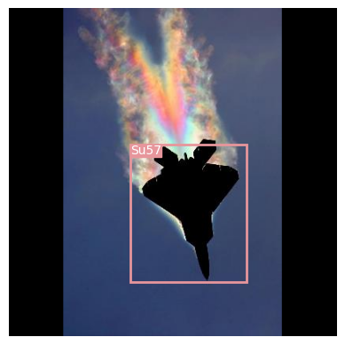
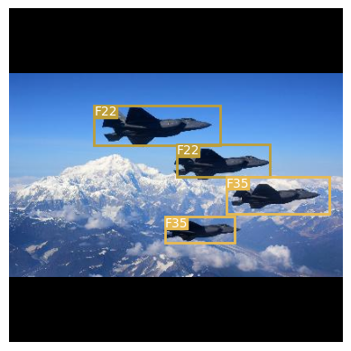
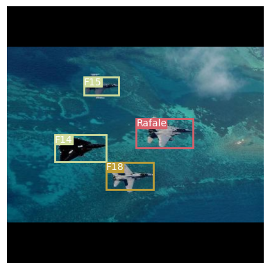
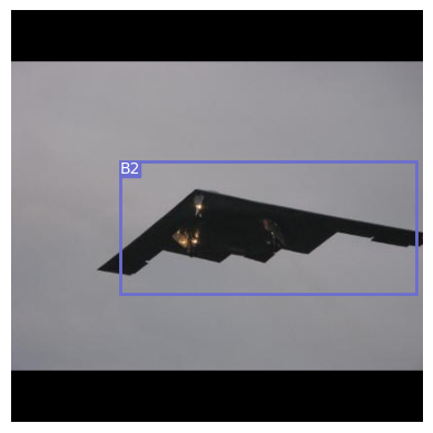
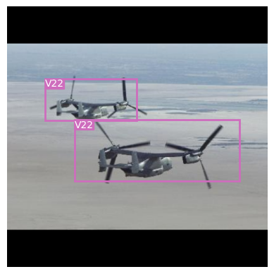
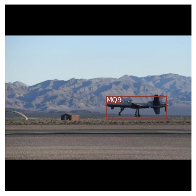
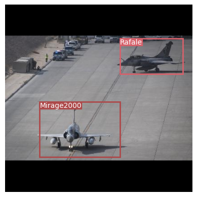
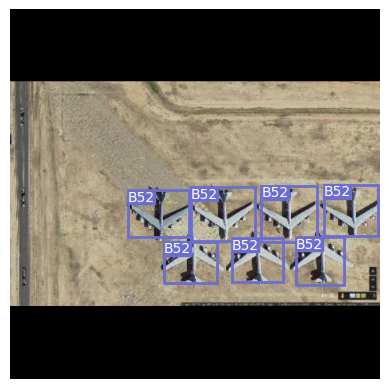
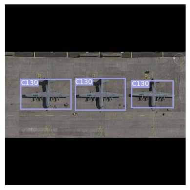
False Positive(wrong class)

F22, F22, F35, F35 → F35, F35, F35, F35
F14, F18, Rafale, F15 → F14, F18, F15, F16
Su57 → F22

NMS(Non-maximum Suppression)

Detection	YOLOv8n	YOLOv8s	YOLOv8m	YOLOv8l	YOLOv8x
v8 + MSE + CA	?	?	8.47	?	?
v8 + CIoU + CA	?	?	8.48	?	?
v8 + SIoU + CA	?	?	?	?	?

GitHub Repository

Military Aircraft Detection with YOLOv8

Reference

Web Link

One-stage object detection : https://machinethink.net/blog/object-detection/
YOLOv5 : https://blog.roboflow.com/yolov5-improvements-and-evaluation/
YOLOv8 : https://blog.roboflow.com/whats-new-in-yolov8/
mAP : https://blog.roboflow.com/mean-average-precision/
SiLU : https://tae-jun.tistory.com/10
Weight Decay, BN : https://blog.janestreet.com/l2-regularization-and-batch-norm/
Focal Loss : https://gaussian37.github.io/dl-concept-focal_loss/
　　　　 　https://woochan-autobiography.tistory.com/929
Cross Entropy : https://sosoeasy.tistory.com/351
DIOU, CIOU : https://hongl.tistory.com/215
QFL, DFL : https://pajamacoder.tistory.com/m/74
YOLOv8 Pytorch : https://github.com/jahongir7174/YOLOv8-pt

Paper

Real-Time Flying Object Detection with YOLOv8 : https://arxiv.org/pdf/2305.09972.pdf
YOLO : https://arxiv.org/pdf/1506.02640.pdf
YOLOv2 : https://arxiv.org/pdf/1612.08242.pdf
YOLOv3 : https://arxiv.org/pdf/1804.02767.pdf
YOLOv4 : https://arxiv.org/pdf/2004.10934.pdf
YOLOv6 : https://arxiv.org/pdf/2209.02976.pdf
YOLOv7 : https://arxiv.org/pdf/2207.02696.pdf
CIoU : https://arxiv.org/abs/1911.08287
QFL, DFL, GFL : https://arxiv.org/abs/2006.04388